How to Create a Budget in Excel (Even if You’re Spectacularly Bad at Excel)


Can’t find a budgeting app you like? Prefer to manually enter your transactions or control the layout of your budget?
A lot of other people do too! That’s why making your own budget spreadsheet is still a common practice for people paying off debt or just trying to spend less than they make.
And because Microsoft Excel has its own app, your budget spreadsheet is no longer bound to your computer.
Why You Need a Monthly Budget Planner
Tracking your income and expenses can be as simple as budgeting every paycheck or as extensive as tracking several years of transactions.
It’s up to you, but I recommend starting small and getting more complex as you improve. Budgeting isn’t something you’re good at right off the bat; it’s a continual lesson in delayed gratification.
If you don’t have access to Excel, you can use the same functions in OpenOffice Calc or Google Sheets, and access your budget using one of their various apps.
A lot of the templates out there are clunky and outdated. Instead of taking the time to conform a template to fit your needs, sometimes the easiest thing to do is make your own.
Even if you wanted to alter a template, editing can get pretty confusing.
So learning how to make a budget in Excel will serve you well no matter what path you choose.
How to Make a Budget in Excel
First, decide what you’d like to track. Here’s a list of 100 expenses to account for in your budget to get you started.
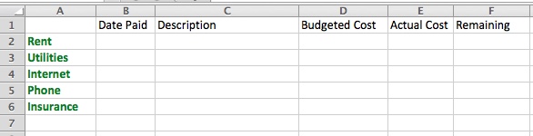
Label rows in column A with the budget categories you’re assigning. Label columns B-F as follows:
- Date Paid
- Description
- Budgeted Cost
- Actual Cost
- Remaining
Once you start inputting data, there are a few Excel shortcuts you should be familiar with.
- AutoSum: Adds numbers in a row, column or both. This is helpful for adding multiple sources of income, all your expenses or even subtracting your expenses from your income. You can perform it with the button in the top bar or the =SUM( formula.
- Insert Multiple Rows: Planned to go out twice this month but find yourself at your third bar… of the night? Adding multiple rows saves you from having to manually shift all your rows and ruining your formulas. You can do this by selecting multiple rows where you want to insert them, then right-clicking and selecting “Insert rows x – y.”
Let’s start giving your budget some character.
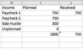
In columns H-J, add the labels “Income,” “Planned” and “Received.” This is where you can add your projected income sources and correct them by tracking your received income.
Once you add all your planned sources of income, highlight them, click the “Sum” button, and then hit enter. That’ll give you your projected total income for the month.
You can do the same with “Received,” but input the formula so you can include the empty cells — something like =SUM(J2:J5).
Go ahead and allot a budgeted cost for all your budget categories. If you’re doing a zero-based budget, while pressing shift, select your first and last budgeted costs. Then hit the “Sum” button. This will give you your total expenses and will change if you adjust the numbers above.
If you want to get real fancy, underneath your planned income, type = and the cell your total expenses are in, e.g., D38, and hit “enter.” Then, AutoSum the two cells. You’ll see in real time where your budget stands.
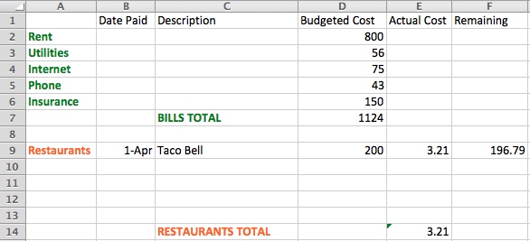
Adding your fixed bills is the easiest part because the budget cost is sure to be the same as your actual. And rent, utilities, etc., are self-explanatory, so you don’t have to enter a description for those. In the “Date Paid” column, you can put the date each bill is due, the date you plan to pay it, or the date it was paid — whatever makes sense to you.

For discretionary spending categories such as groceries, gas, restaurants and entertainment, you just need to add a few more formulas to your budget.
If on the first line of your restaurants budget category you’ve budgeted $200, you can use that same row for your first restaurant transaction entry (which in my case happens to be Taco Bell for $3.21, because my budget loves the dollar menu).
So you’d put $3.21 in “Actual Cost,” e.g., cell E9, and then AutoSum the “Remaining” cell, in this case, F9. You’ll change out the “:” for “-” so that the formula subtracts E9 from D9. It should look something like this: =SUM(D9-E9). This will give you a running tab of what you have left to spend in the restaurants category.
To continue that running tab down the column, you’ll need one more formula. Say my next transaction is $3.11 from Smoothie King because I feel guilty about those dollar menu tacos.
I’d enter the date paid and Smoothie King right under Taco Bell, and then skip the “Budgeted Cost” column (because I don’t need to be reminded how little I have to spend on restaurants).
Under “Actual Cost,” E10, I’d enter $3.11, and then under “Remaining,” F10, I’d input =SUM(F9-E10). That’ll subtract the latest transaction from the latest remaining balance, giving a running total.
With F10 still selected, there will be a little blue box in the lower-right corner of the cell. I’ll click that box and drag it down the column to the last row of the restaurants category.
You’ll see the “Remaining” number in every open row, and it’ll update as you add transactions. I also keep tabs on the total I’ve actually spent, just to be redundant.

Your budget might eventually look something like this (especially if you don’t buy groceries, which I don’t recommend).

Beneath income, I like to compare “Planned Income” with “Budgeted Expenses” to make sure every dollar is going somewhere. You can copy any cell by typing = followed by the cell you want to copy in the selected cell. In this case, the “Planned Income” total is =I6 and the “Budgeted Expenses” total is =D29, so =SUM(I6-D29) is the formula to get the amount left to budget.
The same can be done with received income, =J6, compared with actual expenses, =E30.

But wait, there’s more!
If you’re on a 50/20/30 budget, you can add up your essential living costs, financial goals and personal spending, and put them in a pie chart to track percentages.
To make a pie chart in Excel, select the values and labels you want to include, and select “Pie Chart” (choose “Insert Chart,” under the Charts tab). Voila! Pie chart.
To label slices, right-click the pie and select “Add Data Labels.” It’ll automatically populate the values, so right-click again, select “Format Data Labels”, click “Percentage”, unclick “Value,” and hit “OK.”

Taking Your Excel Budget Template on the Go
To access your Excel budget, you’ll need to create a free Microsoft account and activate OneDrive. Save your budget, and upload it to OneDrive.
Download the Microsoft Excel mobile app, and log in to your Microsoft account. In the “Open” tab select “OneDrive – Personal” and select the file you uploaded your budget to. Click on your spreadsheet and your budget will be available on the go!
To prepare your budget for the next month I suggest creating a new sheet by tapping the “+” button, copying your entire budget and pasting it to the new sheet. If you do this on your computer, you’ll want to update it from the file in OneDrive.
This allows you to not only keep your formulas, but also see what you spent this month to make a realistic budget for the next.
And if the idea of making your own Excel budget template is now utterly horrifying to you, try one of the preloaded budget templates in Excel. With the tips above, you’ll be able to tweak it to your liking without the overwhelm of starting from scratch.
Happy budgeting!
Jen Smith is a staff writer at The Penny Hoarder and gives tips for saving money and paying off debt on Instagram at @savingwithspunk. She religiously budgets every month.